Blackbody Rendering
In between bouts of festive over-eating I added support for blackbody emission to my fluid simulator and thought I'd describe what was involved.
Briefly, a blackbody is an idealised substance that gives off light when heated. Planck's formula describes the intensity of light per-wavelength with units W·sr-1·m-2·m-1 for a given temperature in Kelvins.
Radiance has units W·sr-1·m-2 so we need a way to convert the wavelength dependent power distribution given by Planck's formula to a radiance value in RGB that we can use in our shader / ray-tracer.
The typical way to do this is as follows:
- Integrate Planck's formula against the CIE XYZ colour matching functions (available as part of PBRT in 1nm increments)
- Convert from XYZ to linear sRGB (do not perform gamma correction yet)
- Render as normal
- Perform tone-mapping / gamma correction
We are throwing away spectral information by projecting into XYZ but a quick dimensional analysis shows that now we at least have the correct units (because the integration is with respect to dλ measured in meters the extra m-1 is removed).
I was going to write more about the colour conversion process, but I didn't want to add to the confusion out there by accidentally misusing terminology. Instead here are a couple of papers describing the conversion from Spectrum->RGB and RGB->Spectrum, questions about these come up all the time on various forums and I think these two papers do a good job of providing background and clarifying the process:
- Picture Perfect RGB Rendering Using Spectral Prefiltering and Sharp Color Primaries
- An RGB to Spectrum Conversion for Reflectances
And some more general colour space links:
- The CIE XYZ and xyY Color Spaces by Douglas Kerr (particularly good)
- SIGGRAPH 2010: Color Enhancement and Rendering in Film and Game Production
- Color Space FAQ
Here is a small sample of linear sRGB radiance values for different Blackbody temperatures:
1000K: 1.81e-02, 1.56e-04, 1.56e-04
2000K: 1.71e+03, 4.39e+02, 4.39e+02
4000K: 5.23e+05, 3.42e+05, 3.42e+05
8000K: 9.22e+06, 9.65e+06, 9.65e+06
It's clear from the range of values that we need some sort of exposure control and tone-mapping. I simply picked a temperature in the upper end of my range (around 3000K) and scaled intensities around it before applying Reinhard tone mapping and gamma correction. You can also perform more advanced mapping by taking into account the human visual system adaptation as described in Physically Based Modeling and Animation of Fire.
Again the hardest part was setting up the simulation parameters to get the look you want, here's one I spent at least 4 days tweaking:
Simulation time is ~30s a frame (10 substeps) on a 128^3 grid tracking temperature, fuel, smoke and velocity. Most of that time is spent in the tri-cubic interpolation during advection, I've been meaning to try MacCormack advection to see if it's a net win.
There are some pretty obvious artifacts due to the tri-linear interpolation on the GPU, that would be helped by a higher resolution grid or manually performing tri-cubic in the shader.
Inspired by Kevin Beason's work in progress videos I put together a collection of my own failed tests which I think are quite amusing:
Adventures in Fluid Simulation
I have to admit to being simultaneously fascinated and slightly intimidated by the fluid simulation crowd. I've been watching the videos on Ron Fedkiw's page for years and am still in awe of his results, which sometimes seem little short of magic.
Recently I resolved to write my first fluid simulator and purchased a copy of Fluid Simulation for Computer Graphics by Robert Bridson.
 Like a lot of developers my first exposure to the subject was Jos Stam's stable fluids paper and his more accessible Fluid Dynamics for Games presentation, while the ideas are undeniable great I never came away feeling like I truly understood the concepts or the mathematics behind it.
I'm happy to report that Bridson's book has helped change that. It includes a review of vector calculus in the appendix that is given in a wonderfully straight-forward and concise manner, Bridson takes almost nothing for granted and gives lots of real-world examples which helps for some of the less intuitive concepts.
I'm planning a bigger post on the subject but I thought I'd write a quick update with my progress so far.
I started out with a 2D simulation similar to Stam's demos, having a 2D implementation that you're confident in is really useful when you want to quickly try out different techniques and to sanity check results when things go wrong in 3D (and they will).
Before you write the 3D sim though, you need a way of visualising the data. I spent quite a while on this and implemented a single-scattering model using brute force ray-marching on the GPU.
I did some tests with a procedural pyroclastic cloud model which you can see below, this runs at around 25ms on my MacBook Pro (NVIDIA 320M) but you can dial the sample counts up and down to suit:
Here's a simplified GLSL snippet of the volume rendering shader, it's not at all optimised apart from some branches to skip over empty space and an assumption that absorption varies linearly with density:
uniform sampler3D g_densityTex;
uniform vec3 g_lightPos;
uniform vec3 g_lightIntensity;
uniform vec3 g_eyePos;
uniform float g_absorption;

void main()
{
    // diagonal of the cube
    const float maxDist = sqrt(3.0);

    const int numSamples = 128;
    const float scale = maxDist/float(numSamples);

    const int numLightSamples = 32;
    const float lscale = maxDist / float(numLightSamples);

    // assume all coordinates are in texture space
    vec3 pos = gl_TexCoord[0].xyz;
    vec3 eyeDir = normalize(pos-g_eyePos)*scale;

    // transmittance
    float T = 1.0;
    // in-scattered radiance
    vec3 Lo = vec3(0.0);

    for (int i=0; i < numSamples; ++i)
    {
        // sample density
        float density = texture3D(g_densityTex, pos).x;

        // skip empty space
        if (density > 0.0)
        {
            // attenuate ray-throughput
            T *= 1.0-density*scale*g_absorption;
            if (T <= 0.01)
                break;

            // point light dir in texture space
            vec3 lightDir = normalize(g_lightPos-pos)*lscale;

            // sample light
            float Tl = 1.0; // transmittance along light ray
            vec3 lpos = pos + lightDir;

            for (int s=0; s < numLightSamples; ++s)
            {
                float ld = texture3D(g_densityTex, lpos).x;
                Tl *= 1.0-g_absorption*lscale*ld;

                if (Tl <= 0.01)
                    break;

                lpos += lightDir;
            }

            vec3 Li = g_lightIntensity*Tl;

            Lo += Li*T*density*scale;
        }

        pos += eyeDir;
    }

    gl_FragColor.xyz = Lo;
    gl_FragColor.w = 1.0-T;
}
I'm pretty sure there's a whole post on the ways this could be optimised but I'll save that for next time. Also this example shader doesn't have any wavelength dependent variation. Making your absorption coefficient different for each channel looks much more interesting and having a different coefficient for your primary and shadow rays also helps, you can see this effect in the videos.
To create the cloud like volume texture in OpenGL I use a displaced distance field like this (see the SIGGRAPH course for more details):
// create a volume texture with n^3 texels and base radius r
GLuint CreatePyroclasticVolume(int n, float r)
{
    GLuint texid;
    glGenTextures(1, &texid);

    GLenum target = GL_TEXTURE_3D;
    GLenum filter = GL_LINEAR;
    GLenum address = GL_CLAMP_TO_BORDER;

    glBindTexture(target, texid);

    glTexParameteri(target, GL_TEXTURE_MAG_FILTER, filter);
    glTexParameteri(target, GL_TEXTURE_MIN_FILTER, filter);

    glTexParameteri(target, GL_TEXTURE_WRAP_S, address);
    glTexParameteri(target, GL_TEXTURE_WRAP_T, address);
    glTexParameteri(target, GL_TEXTURE_WRAP_R, address);

    glPixelStorei(GL_UNPACK_ALIGNMENT, 1);

    byte *data = new byte[n*n*n];
    byte *ptr = data;

    float frequency = 3.0f / n;
    float center = n / 2.0f + 0.5f;

    for(int x=0; x < n; x++)
    {
        for (int y=0; y < n; ++y)
        {
            for (int z=0; z < n; ++z)
            {
                float dx = center-x;
                float dy = center-y;
                float dz = center-z;

                float off = fabsf(Perlin3D(x*frequency,
                               y*frequency,
                               z*frequency,
                               5,
                               0.5f));

                float d = sqrtf(dx*dx+dy*dy+dz*dz)/(n);

                *ptr++ = ((d-off) < r)?255:0;
            }
        }
    }

    // upload
    glTexImage3D(target,
                 0,
                 GL_LUMINANCE,
                 n,
                 n,
                 n,
                 0,
                 GL_LUMINANCE,
                 GL_UNSIGNED_BYTE,
                 data);

    delete[] data;

    return texid;
}
An excellent introduction to volume rendering is the SIGGRAPH 2010 course, Volumetric Methods in Visual Effects and Kyle Hayward's Volume Rendering 101 for some GPU specifics.
Once I had the visualisation in place, porting the fluid simulation to 3D was actually not too difficult. I spent most of my time tweaking the initial conditions to get the smoke to behave in a way that looks interesting, you can see one of my more successful simulations below:
Currently the simulation runs entirely on the CPU using a 128^3 grid with monotonic tri-cubic interpolation and vorticity confinement as described in Visual Simulation of Smoke by Fedkiw. I'm fairly happy with the result but perhaps I have the vorticity confinement cranked a little high.
Nothing is optimised so its running at about 1.2s a frame on my 2.66ghz Core 2 MacBook.
Future work is to port the simulation to OpenCL and implement some more advanced features. Specifically I'm interested in A Vortex Particle Method for Smoke, Water and Explosions which Kevin Beason describes on his fluid page (with some great videos).
On a personal note, I resigned from LucasArts a couple of weeks ago and am looking forward to some time off back in New Zealand with my family and friends. Just in time for the Kiwi summer!
Links
Tracing
Gregory Pakosz reminded me to write a follow up on my path tracing efforts since my last post on the subject.
It's good timing because the friendly work-place competition between Tom and me has been in full swing. The great thing about ray tracing is that there are many opportunities for optimisation at all levels of computation. This keeps you "hooked" by constantly offering decent speed increases for relatively little effort.
Tom had an existing BIH (bounding interval hierarchy) implementation that was doing a pretty good job, so I had some catching up to do. Previously I had a positive experience using a BVH (AABB tree) in a games context so decided to go that route.
Our benchmark scene was Crytek's Sponza with the camera positioned in the center of the model looking down the z-axis. This might not be the most representative case but was good enough for comparing primary ray speeds.
Here's a rough timeline of the performance progress (all timings were taken from my 2.6ghz i7 running 8 worker threads):
| Optimisation | Rays/second |
|---|---|
| Baseline (median split) | 91246 |
| Tweak compiler settings (/fp:fast /sse2 /Ot) | 137486 |
| Non-recursive traversal | 145847 |
| Traverse closest branch first | 146822 |
| Surface area heuristic | 1.27589e+006 |
| Surface area heuristic (exhaustive) | 1.9375e+006 |
| Optimized ray-AABB | 2.14232e+006 |
| VS2008 to VS2010 | 2.47746e+006 |
You can see the massive difference tree quality has on performance. What I found surprising though was the effect switching to VS2010 had, 15% faster is impressive for a single compiler revision.
I played around with a quantized BVH which reduced node size from 32 bytes to 11 but I couldn't get the decrease in cache traffic to outweigh the cost in decoding the nodes. If anyone has had success with this I'd be interested in the details.
Algorithmically it is a uni-directional path tracer with multiple importance sampling. Of course importance sampling doesn't make individual samples faster but allows you to take less total samples than you would have to otherwise.
So, time for some pictures:
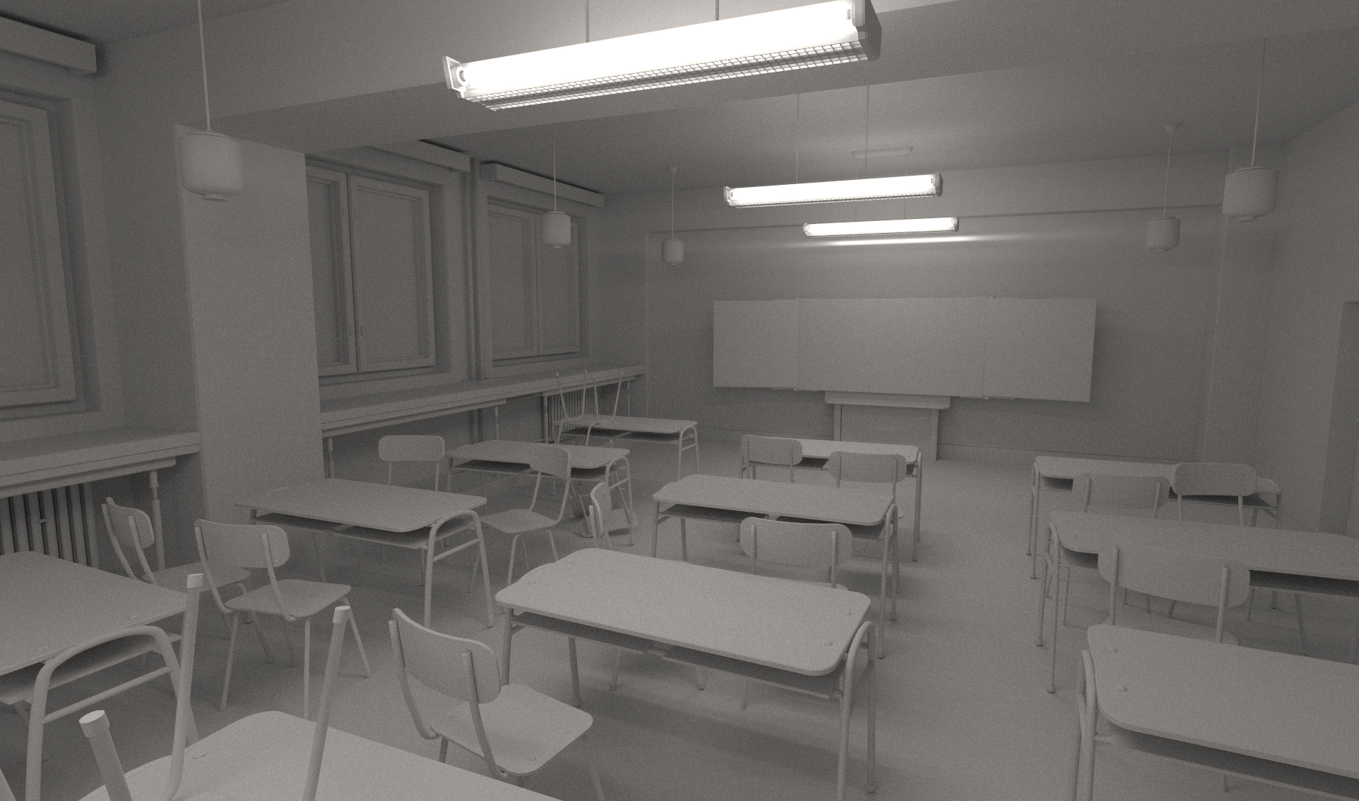
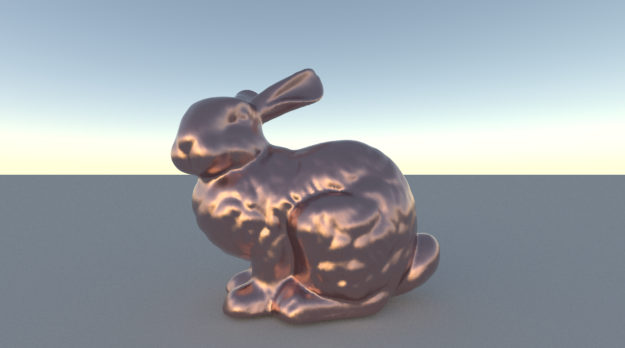
Despite being the lowest poly models, Sponza (200k triangles) and the classroom (250k triangles) were by far the most difficult for the renderer; they both took 10+ hours and still have visible noise. In contrast the gold statuette (10 million triangles) took only 20 mins to converge!
This is mainly because the architectural models have a mixture of very large and very small polygons which creates deep trees with large nodes near the root. I think a kd-tree which splits or duplicates primitives might be more effective in this case.
A fun way to break your spatial hierarchy is simply to add a ground plane. Until I performed an exhaustive split search adding a large two triangle ground plane could slow down tracing by as much as 50%.
Of course these numbers are peanuts compared to what people are getting with GPU or SIMD packet tracers, Timo Aila reports speeds of 142 million rays/second on similar scenes using a GPU tracer in this paper.
Writing a path tracer has been a great education for me and I would encourage anyone interested in getting a better grasp on computer graphics to get a copy of PBRT and have a go at it. It's easy to get started and seeing the finished product is hugely rewarding.
Model credits:
Sponza - Crytek
Classroom - LuxRender
Thai Statuette, Dragon, Bunny, Lucy - Stanford scanning repository
Faster Fog
Cedrick at Lucas suggested some nice optimisations for the in-scattering equation I posted last time.
I had left off at:
\[L_{s} = \frac{\sigma_{s}I}{v}( \tan^{-1}\left(\frac{d+b}{v}\right) - \tan^{-1}\left(\frac{b}{v}\right) )\]
But we can remove one of the two inverse trigonometric functions by using the following identity:
\[\tan^{-1}x - \tan^{-1}y = \tan^{-1}\frac{x-y}{1+xy}\]
Which simplifies the expression for $L_{s}$ to:
\[L_{s} = \frac{\sigma_{s}I}{v}( \tan^{-1}\frac{x-y}{1+xy} )\]
With $x$ and $y$ being replaced by:
\[\begin{array}{lcl} x = \frac{d+b}{v} \\ y = \frac{b}{v}\end{array}\]
So the updated GLSL snippet looks like:
float InScatter(vec3 start, vec3 dir, vec3 lightPos, float d)
{
   vec3 q = start - lightPos;

   // calculate coefficients
   float b = dot(dir, q);
   float c = dot(q, q);
   float s = 1.0f / sqrt(c - b*b);

   // after a little algebraic re-arrangement
   float x = d*s;
   float y = b*s;
   float l = s * atan( (x) / (1.0+(x+y)*y));

   return l;
}
Of course it's always good to verify your 'optimisations', ideally I would take GPU timings but next best is to run it through NVShaderPerf and check the cycle counts:
Original (2x atan()):
Fragment Performance Setup: Driver 174.74, GPU G80, Flags 0x1000
Results 76 cycles, 10 r regs, 2,488,320,064 pixels/s
Updated (1x atan())
Fragment Performance Setup: Driver 174.74, GPU G80, Flags 0x1000
Results 55 cycles, 8 r regs, 3,251,200,103 pixels/s
A tasty 25% reduction in cycle count!
Another idea is to use an approximation of atan(), Robin Green has some great articles about faster math functions where he discusses how you can range reduce to 0-1 and approximate using minimax polynomials.
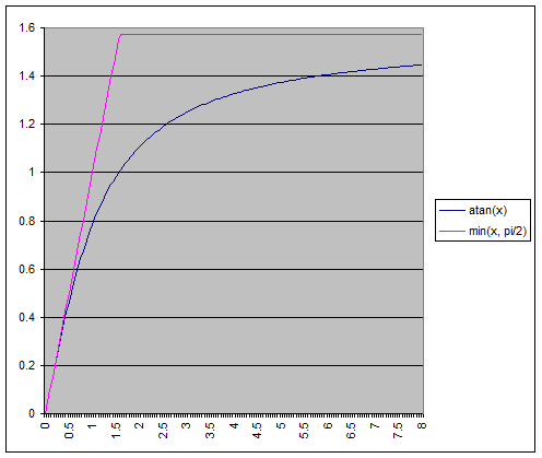
My first attempt was much simpler, looking at it's graph we can see that atan() is almost linear near 0 and asymptotically approaches pi/2.
Perhaps the simplest approximation we could try would be something like:
\[\tan^{-1}(x) \approx min(x, \frac{\pi}{2})\]
Which looks like:
float atanLinear(float x)
{
   return clamp(x, -0.5*kPi, 0.5*kPi);
}

// Fragment Performance Setup: Driver 174.74, GPU G80, Flags 0x1000
// Results 34 cycles, 8 r regs, 4,991,999,816 pixels/s
Pretty ugly, but even though the maximum error here is huge (~0.43 relative), visually the difference is surprisingly small.
Still I thought I'd try for something more accurate, I used a 3rd degree minimax polynomial to approximate the range 0-1 which gave something practically identical to atan() for my purposes (~0.0052 max relative error):
float MiniMax3(float x)
{
   return ((-0.130234*x - 0.0954105)*x + 1.00712)*x - 0.00001203333;
}

float atanMiniMax3(float x)
{
   // range reduction
   if (x < 1)
      return MiniMax3(x);
   else
      return kPi*0.5 - MiniMax3(1.0/x);
}

// Fragment Performance Setup: Driver 174.74, GPU G80, Flags 0x1000
// Results 40 cycles, 8 r regs, 4,239,359,951 pixels/s
Disclaimer: This isn't designed as a general replacement for atan(), for a start it doesn't handle values of x < 0 and it hasn't had anywhere near the love put into other approximations you can find online (optimising for floating point representations for example).
As a bonus I found that putting the polynomial evaluation into Horner form shaved 4 cycles from the shader.
Cedrick also had an idea to use something a little different:
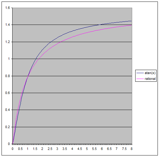
\[\tan^{-1}(x) \approx \frac{\pi}{2}\left(\frac{kx}{1+kx}\right)\]
This might look familiar to some as the basic Reinhard tone mapping curve! We eyeballed values for k until we had one that looked close (you can tell I'm being very rigorous here), in the end k=1 was close enough and is one cycle faster :)
float atanRational(float x)
{
   return kPi*0.5*x / (1.0+x);
}

// Fragment Performance Setup: Driver 174.74, GPU G80, Flags 0x1000
// Results 34 cycles, 8 r regs, 4,869,120,025 pixels/s
To get it down to 34 cycles we had to expand out the expression for x and perform some more grouping of terms which shaved another cycle and a register off it. I was surprised to see the rational approximation be so close in terms of performance to the linear one, I guess the scheduler is doing a good job at hiding some work there.
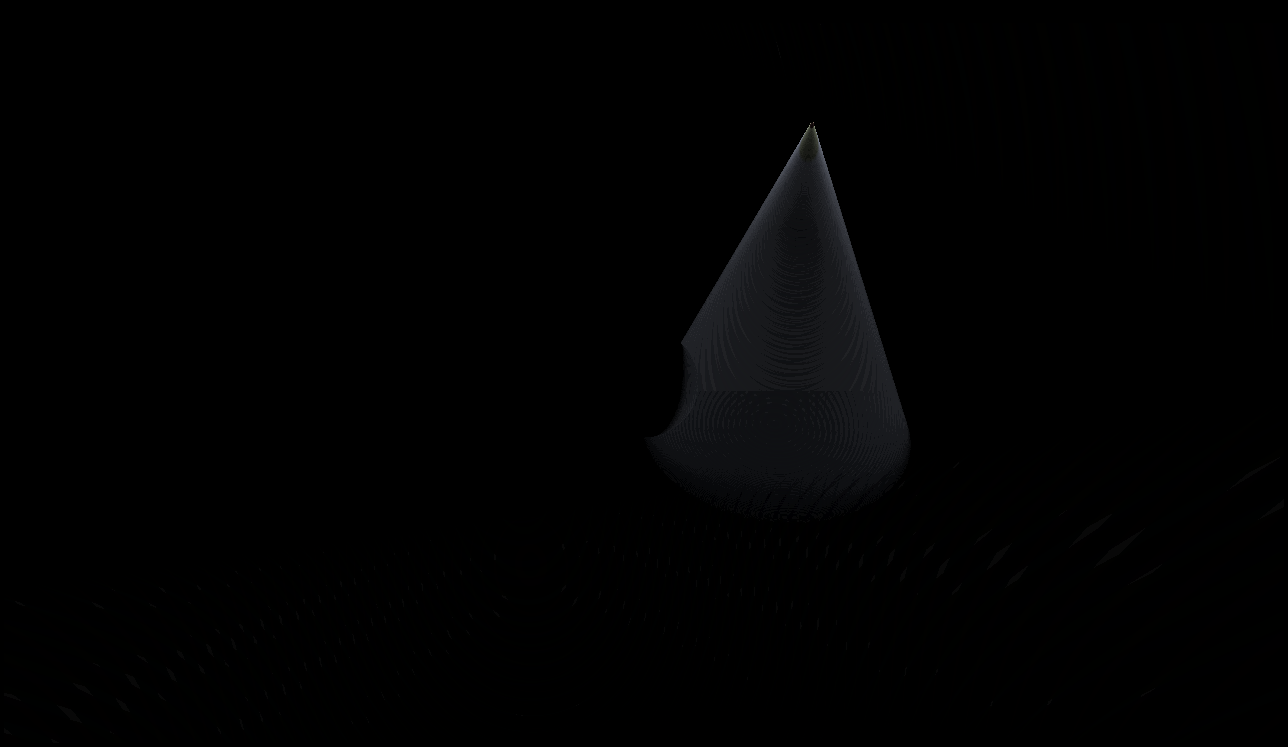
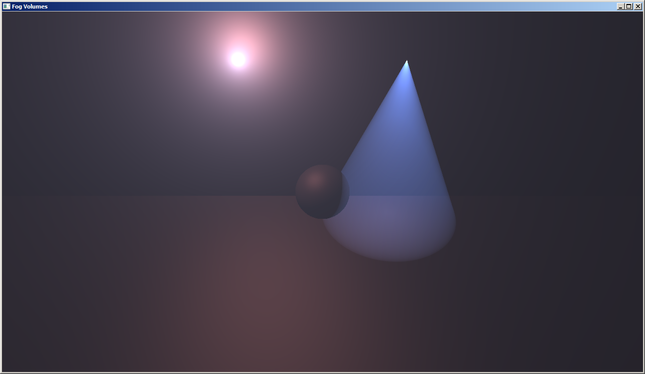
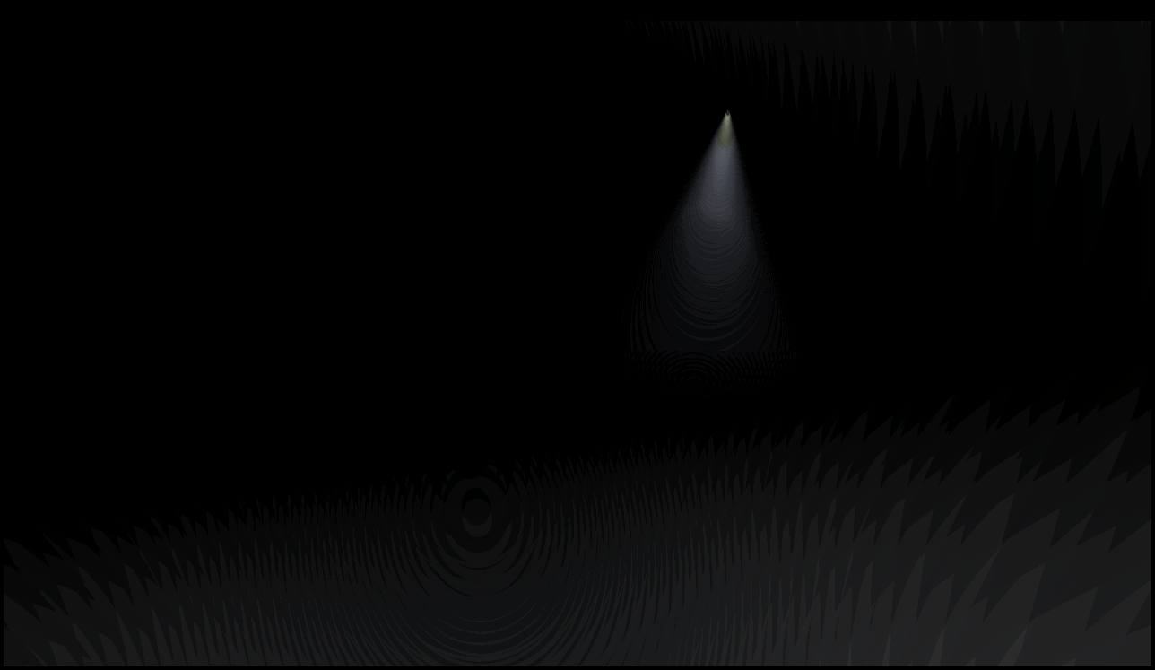
In the end all three approximations gave pretty good visual results:
Original (cycle count 76):
MiniMax3, Error 8x (cycle count 40):
Rational, Error 8x (cycle count 34):
Linear, Error 8x (cycle count 34):
Links:
http://realtimecollisiondetection.net/blog/?p=9
http://www.research.scea.com/gdc2003/fast-math-functions.html
In-Scattering Demo
This demo shows an analytic solution to the differential in-scattering equation for light in participating media. It's a similar but simplified version of equations found in [1], [2] and as I recently discovered [3]. However I thought showing the derivation might be interesting for some out there, plus it was a good excuse for me to brush up on my \(\LaTeX\).
You might notice I also updated the site's theme, unfortunately you need a white background to make wordpress.com LaTeX rendering play nice with RSS feeds (other than that it's very convenient).
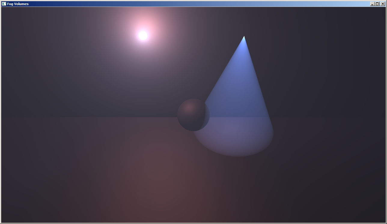
The demo uses GLSL and shows point and spot lights in a basic scene with some tweakable parameters:
Background
Given a view ray defined as:
\[\mathbf{x}(t) = \mathbf{p} + t\mathbf{d}\]
We would like to know the total amount of light scattered towards the viewer (in-scattered) due to a point light source. For the purposes of this post I will only consider single scattering within isotropic media.
The differential equation that describes the change in radiance due to light scattered into the view direction inside a differential volume is given in PBRT (p578), if we assume equal scattering in all directions we can write it as:
\[dL_{s}(t) = \sigma_{s}L_{i}(t)\,dt\]
Where \(\sigma_{s}\) is the scattering probability which I will assume includes the normalization term for an isotropic phase funtion of \(\frac{1}{4pi}\). For a point light source at distance d with intensity I we can calculate the radiant intensity at a receiving point as:
\[L_{i} = \frac{I}{d^2}\]
Plugging in the equation for a point along the view ray we have:
\[L_{i}(t) = \frac{I}{|\mathbf{x}(t)-\mathbf{s}|^2}\]
Where s is the light source position. The solution to (1) is then given by:
\[L_{s} = \int_{0}^{d} \sigma_{s}L_{i}(t) \, dt\]
\[L_{s} = \int_{0}^{d} \frac{\sigma_{s}I}{|\mathbf{x}(t)-\mathbf{s}|^2}\,dt\]
To find this integral in closed form we need to expand the distance calculation in the denominator into something we can deal with more easily:
\[L_{s} = \sigma_{s}I\int_0^d{\frac{dt}{(\mathbf{p} + t\mathbf{d} - \mathbf{s})\cdot(\mathbf{p} + t\mathbf{d} - \mathbf{s})}}\]
Expanding the dot product and gathering terms, we have:
\[L_{s} = \sigma_{s}I\int_{0}^{d}\frac{dt}{(\mathbf{d}\cdot\mathbf{d})t^2 + 2(\mathbf{m}\cdot\mathbf{d})t + \mathbf{m}\cdot\mathbf{m} }\]
Where \(\mathbf{m} = (\mathbf{p}-\mathbf{s})\).
Now we have something a bit more familiar, because the direction vector is unit length we can remove the coefficient from the quadratic term and we have:
\[L_{s} = \sigma_{s}I\int_{0}^{d}\frac{dt}{t^2 + 2bt + c}\]
At this point you could look up the integral in standard tables but I'll continue to simplify it for completeness. Completing the square we obtain:
\[L_{s} = \sigma_{s}I\int_{0}^{d}\frac{dt}{ (t^2 + 2bt + b^2) + (c-b^2)}\]
Making the substitution (u = (t + b)), (v = (c-b2){1/2}) and updating our limits of integration, we have:
\[L_{s} = \sigma_{s}I\int_{b}^{b+d}\frac{du}{ u^2 + v^2}\]
\[L_{s} = \sigma_{s}I \left[ \frac{1}{v}\tan^{-1}\frac{u}{v} \right]_b^{b+d}\]
Finally giving:
\[L_{s} = \frac{\sigma_{s}I}{v}( \tan^{-1}\frac{d+b}{v} - \tan^{-1}\frac{b}{v} )\]
This is what we will evaluate in the pixel shader, here's the GLSL snippet for the integral evaluation (direct translation of the equation above):
float InScatter(vec3 start, vec3 dir, vec3 lightPos, float d)
{
// light to ray origin
vec3 q = start - lightPos;

// coefficients
float b = dot(dir, q);
float c = dot(q, q);

// evaluate integral
float s = 1.0f / sqrt(c - b*b);
float l = s * (atan( (d + b) * s) - atan( b*s ));

return l;
}
Where d is the distance traveled, computed by finding the entry / exit points of the ray with the volume.
To make the effect more interesting it is possible to incorporate a particle system, I apply the same scattering shader to each particle and treat it as a thin slab to obtain an approximate depth, then simply multiply by a noise texture at the end.
Optimisations
- As it is above the code only supports lights with infinite extent, this implies drawing the entire frame for each light. It would be possible to limit it to a volume but you'd want to add a falloff to the effect to avoid a sharp transition at the boundary.
- Performing the full evaluation per-pixel for the particles is probably unnecessary, doing it at a lower frequency, per-vertex or even per-particle would probably look acceptable.
Notes
- Generally objects appear to have wider specular highlights and more ambient lighting in the presence of particpating media. [1] Discusses this in detail but you can fudge it by lowering the specular power in your materials as the scattering coefficient increases.
- According to Rayliegh scattering blue light at the lower end of the spectrum is scattered considerably more than red light. It's simple to account for this wavelength dependence by making the scattering coefficient a constant vector weighted towards the blue component. I found this helps add to the realism of the effect.
- I'm curious to know how the torch light was done in Alan Wake as it seems to be high quality (not just billboards) with multiple light shafts.. maybe someone out there knows?
References
- Sun, B., Ramamoorthi, R., Narasimhan, S. G., and Nayar, S. K. 2005. A practical analytic single scattering model for real time rendering.
- Wenzel, C. 2006. Real-time atmospheric effects in games.
- Zhou, K., Hou, Q., Gong, M., Snyder, J., Guo, B., and Shum, H. 2007. Fogshop: Real-Time Design and Rendering of Inhomogeneous, Single-Scattering Media.
- Engelhardt, T. and Dachsbacher, C. 2010. Epipolar sampling for shadows and crepuscular rays in participating media with single scattering.
- Volumetric Shadows using Polygonal Light Volumes
Threading Fun
So we had an interesting threading bug at work today which I thought I'd write up here as I hadn't seen this specific problem before (note I didn't write this code, I just helped debug it). The set up was a basic single producer single consumer arrangement something like this:
#include <Windows.h>
#include <cassert>

volatile LONG gAvailable = 0;

// thread 1
DWORD WINAPI Producer(LPVOID)
{
    while (1)
    {
        InterlockedIncrement(&gAvailable);
    }
}

// thread 2
DWORD WINAPI Consumer(LPVOID)
{
    while (1)
    {
        // pull available work with a limit of 5 items per iteration
        LONG work = min(gAvailable, 5);

        // this should never fire.. right?
        assert(work <= 5);

        // update available work
        InterlockedExchangeAdd(&gAvailable, -work);
    }
}

int main(int argc, char* argv[])
{
    HANDLE h[2];

    h[0] = CreateThread(0, 0, Consumer, NULL, 0, 0);
    h[1] = CreateThread(0, 0, Producer, NULL, 0, 0);

    WaitForMultipleObjects(2, h, TRUE, INFINITE);

    return 0;
}
So where's the problem? What would make the assert fire?
We triple-checked the logic and couldn't see anything wrong (it was more complicated than the example above so there were a number of possible culprits) and unlike the example above there were no asserts, just a hung thread at some later stage of execution.
Unfortunately the bug reproduced only once every other week so we knew we had to fix it while I had it in a debugger. We checked all the relevant in-memory data and couldn't see any that had obviously been overwritten ("memory stomp" is usually the first thing called out when these kinds of bugs show up).
It took us a while but eventually we checked the disassembly for the call to min(). Much to our surprise it was performing two loads of gAvailable instead of the one we had expected!
This happened to be on X360 but the same problem occurs on Win32, here's the disassembly for the code above (VS2010 Debug):
// calculate available work with a limit of 5 items per iteration
LONG work = min(gAvailable, 5);

// (1) read gAvailable, compare against 5
002D1457  cmp         dword ptr [gAvailable (2D7140h)],5
002D145E  jge         Consumer+3Dh (2D146Dh)

// (2) read gAvailable again, store on stack
002D1460  mov         eax,dword ptr [gAvailable (2D7140h)]
002D1465  mov         dword ptr [ebp-0D0h],eax
002D146B  jmp         Consumer+47h (2D1477h)
002D146D  mov         dword ptr [ebp-0D0h],5

// (3) store gAvailable from (2) in 'work'
002D1477  mov         ecx,dword ptr [ebp-0D0h]
002D147D  mov         dword ptr [work],ecx
The question is what happens between (1) and (2)? Well the answer is that any other thread can add to gAvailable, meaning that the stored value at (3) is now > 5.
In this case the simple solution was to read gAvailable outside of the call to min():
// pull available work with a limit of 5 items per iteration
LONG available = gAvailable;
LONG work = min(available, 5);
Maybe this is obvious to some people but it sure caused me and some smart people a headache for a few hours :)
Note that you may not see the problem in some build configurations depending on whether or not the compiler generates code to perform the second read of the variable after the comparison. As far as I know there are no guarantees about what it may or may not do in this case, FWIW we had the problem in a release build with optimisations enabled.
Big props to Tom and Ruslan at Lucas for helping track this one down.
GOW III: Shadows
I checked out this session at GDC today - I'll try and sum up the main takeaways (at least for me):
- Artist controlled cascaded shadow maps, each cascade is accumulated into a 'white buffer' (new term coined?) in deferred style passes using standard PCF filtering
- Shadow accumulation pass re-projects world space position from an FP32 depth buffer (separate from the main depth buffer). The motivation for the separate depth buffer is performance so I assume they store linear depth which means they can reconstruct the world position using just a single multiply-add (saving a reciprocal).
- They have the ability to tile individual cascades to achieve arbitrary levels of sampling within a fixed size memory (render cascade tile, apply into white buffer, repeat)
- Often up to 9 mega-texel resolution used for in game scenes
- White buffer is blended to using MIN blend mode to avoid double darkening (old school)
- Invisible 'caster only' geometry to make baked shadows match on dynamic objects
- Stencil bits used to mask off baked geometry, fore-ground, back-ground characters
The most interesting part (in my opinion) was the optimisation work, Ben creates a light direction aligned 8x8x4 grid that he renders extruded bounding spheres into (on the SPUs). Each cell records whether or not it is in shadow and the rough bounds of that shadow. To take advantage of this information the accumulation pass (where the expensive filtering is done) breaks the screen up into tiles, checks the tile against the volume and adjusts it's depth and 2D bounds accordingly, potentially rejecting entire tiles.
Looking forward to the the rest of the talks, this is my first year at GDC and it's pretty great :)
Stochastic Pruning (2)
A quick update for anyone who was having problems running my stochastic pruning demo on NVIDIA cards, I've updated the demo with a fix (I had forgotten to disable a vertex array).
While I was at it I added some grass:
The grass uses stochastic pruning but still generates a lot of geometry, it's just one grass tile flipped around and rendered multiple times. I wanted to see if it would be practical for games to render grass using pure geometry but really you'd need to be much more aggressive with the LOD (Update: apparently the same technique was used in Flower, see comments).
Kevin Boulanger has done some impressive real time grass rendering using 3 levels of detail with transitions. Cool stuff and quite practical by the looks of it.
Stochastic Pruning for Real-Time LOD
Rendering plants efficiently has always been a challenge in computer graphics, a relatively new technique to address this is Pixar's stochastic pruning algorithm. Originally developed for rendering the desert scenes in Cars, Weta also claim to have used the same technique on Avatar.
Although designed with offline rendering in mind it maps very naturally to the GPU and real-time rendering. The basic algorithm is this:
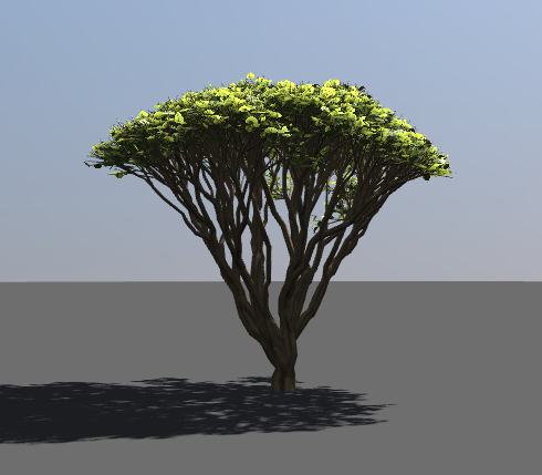
- Build your mesh of N elements (in the case of a tree the elements would be leaves, usually represented by quads)
- Sort the elements in random order (a robust way of doing this is to use the Fisher-Yates shuffle)
- Calculate the proportion U of elements to render based on distance to the object.
- Draw N*U unpruned elements with area scaled by 1/U
So putting this onto the GPU is straightforward, pre-shuffle your index buffer (element wise), when you come to draw you can calculate the unpruned element count using something like:
// calculate scaled distance to viewer
float z = max(1.0f, Length(viewerPos-objectPos)/pruneStartDistance);
// distance at which half the leaves will be pruned
float h = 2.0f;
// proportion of elements unpruned
float u = powf(z, -Log(h, 2));
// actual element count
int m = ceil(numElements * u);
// scale factor
float s = 1.0f / u;
Then just submit a modified draw call for m quads:
glDrawElements(GL_QUADS, m*4, GL_UNSIGNED_SHORT, 0);
The scale factor computed above preserves the total global surface area of all elements, this ensures consistent pixel coverage at any distance. The scaling by area can be performed efficiently in the vertex shader meaning no CPU involvement is necessary (aside from setting up the parameters of course). In a basic implementation you would see elements pop in and out as you change distance but this can be helped by having a transition window that scales elements down before they become pruned (discussed in the original paper).
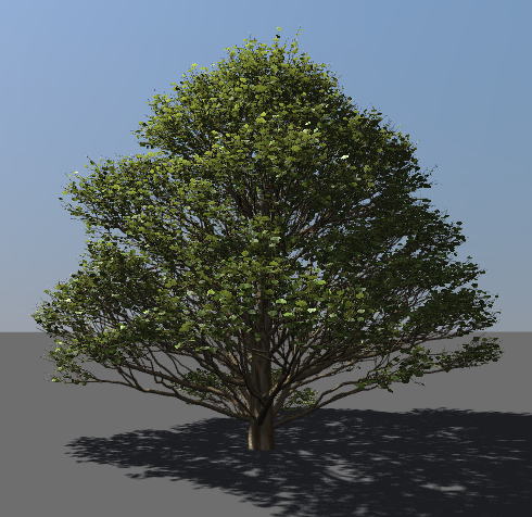
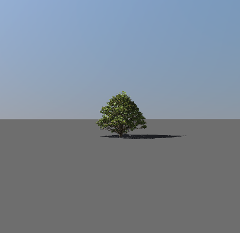
Billboards still have their place but it seems like this kind of technique could have applications for many effects, grass and particle systems being obvious ones.
I've updated my previous tree demo with an implementation of stochastic pruning and a few other changes:
- Fixed some bugs with ATI driver compatability
- Preetham based sky-dome
- Optimised shadow map generation
- Some new example plants
- Tweaked leaf and branch shaders
You can download the demo here
I use the Self-organising tree models for image synthesis algorithm (from SIGGRAPH09) to generate the trees which I have posted about previously.
While I was researching I also came across Physically Guided Animation of Trees from Eurographics 2009, they have some great videos of real-time animated trees.
I've also posted my collection of plant modelling papers onto Mendeley (great tool for organising pdfs!).
Sky
I had been meaning to implement Preetham's analytic sky model ever since I first came across it years ago. Well I finally got around to it and was pleased to find it's one of those few papers that gives you pretty much everything you need to put together an implementation (although with over 50 unique constants you need to be careful with your typing).
I integrated it into my path tracer which made for some nice images:
Also a small video.
It looks like the technique has been surpassed now by Precomputed Atmospheric Scattering but it's still useful for generating environment maps / SH lights.
I also fixed a load of bugs in my path tracer, I was surprised to find that on my new i7 quad-core (8 logical threads) renders with 8 worker threads were only twice as fast as with a single worker, given the embarrassingly parallel nature of path-tracing you would expect at least a factor of 4 decrease in render time.
It turns out the problem was contention in the OS allocator, as I allocate BRDF objects per-intersection there was a lot of overhead there (more than I had expected). I added a per-thread memory arena where each worker thread has a pool of memory to allocate from linearly during a trace, allocations are never freed and the pool is just reset per-path.
This had the following effect on render times:
1 thread:  128709ms->35553ms  (3.6x faster)
8 threads: 54071ms->8235ms   (6.5x faster!)
You might also notice that the total speed up is not linear with the number of workers. It tails off as the 4 'real' execution units are used up, so hyper-threading doesn't seem to be too effective here, I suspect this is due to such simple scenes not providing enough opportunity for swapping the thread states.
The HT numbers seems to roughly agree with what people are reporting on the Ompf forums (~20% improvement).


