XPBD slides and stiffness
The slides for my talk on XPBD are now up on the publications page, or available here.
I spoke to someone who had already implemented the method and who was surprised to find they needed to use very small compliance values in the range of 10
The reason for this is that, unlike stiffness in PBD, compliance in XPBD has a direct correspondence to engineering stiffness, i.e.: Young's modulus. Most real-world materials have a Young's modulus of several GPa (
Below are some stiffness values for some common materials, I have listed the compliance in the right hand column, which is of course just the reciprocal of the stiffness.
| Material | Stiffness (N/m^2) | Compliance (m^2/N) |
|---|---|---|
| Concrete | 25.0 x 10⁹ | 0.04 x 10⁻⁹ |
| Wood | 6.0 x 10⁹ | 0.16 x 10⁻⁹ |
| Leather | 1.0 x 10⁸ | 1.0 x 10⁻⁸ |
| Tendon | 5.0 x 10⁷ | 0.2 x 10⁻⁷ |
| Rubber | 1.0 x 10⁶ | 1.0 x 10⁻⁶ |
| Muscle | 5.0 x 10³ | 0.2 x 10⁻³ |
| Fat | 1.0 x 10³ | 1.0 x 10⁻³ |
Note that for deformable materials, like soft tissue, the material stiffness depends heavily on strain. In the case of muscle it may become up to three orders of magnitude stiffer as it is stretched, even the surrounding temperature can have a large impact on these materials. The values listed here should only be used as a rough guide for a material under low strain.
This is probably not a very convenient range for artists to work with, so it can make sense to expose a parameter in the [0,1] range, map it to the desired stiffness range, and then take the reciprocal to obtain compliance.
Sources
XPBD
Anyone who has worked with Position-Based Dynamics (PBD) in production will know that the constraint stiffness is heavily dependent on the number of iterations performed by the solver. Regardless of how you set the stiffness coefficients, the solver will converge to an infinitely stiff solution given enough iterations.
We have a new paper that solves this iteration count and time step dependent stiffness with a very small addition to the original algorithm. Here is the abstract:
We address the long-standing problem of iteration count and time-step dependent constraint stiffness in position-based dynamics (PBD). We introduce a simple extension to PBD that allows it to accurately and efficiently simulate arbitrary elastic and dissipative energy potentials in an implicit manner. In addition, our method provides constraint force estimates, making it applicable to a wider range of applications, such as those requiring haptic user-feedback. We compare our algorithm to more expensive non-linear solvers and find it produces visually similar results while maintaining the simplicity and robustness of the PBD method.
The method is derived from an implicit integration scheme, and produces results very close to those given by more complex Newton-based solvers, as you can see in the submission video:
I will be presenting the paper at Motion in Games (MIG) in San Francisco next month. If you're in the area you should attend, these smaller conferences are usually very nice.
New SIGGRAPH paper
Just a quick note to say that the pre-print for our paper on particle physics for real-time applications is now available. Visit the project page for all the downloads, or check out the submission video below:
The paper contains most of the practical knowledge and insight about Position-Based Dynamics that I gained while developing Flex. In addition, it introduces a few new features such as implicit friction and smoke simulation.
As noted in the paper, unified solvers are common in offline VFX, but are relatively rare in games. In fact, it was my experience at Rocksteady working on Batman: Arkham Asylum that helped inspire this work. The Batman universe has all these great characters with unique special powers, and I think a tool like this would have found many applications (e.g.: a Clayface boss fight). Particle based methods have their limitations, and traditional rigid-body physics engines will still be important, but I think frameworks like this can be a great addition to the toolbox.
FLEX
FLEX is the name of the new GPU physics solver I have been working on at NVIDIA. It was announced at the Montreal editor's day a few weeks ago, and today we have released some more information in the form of a video trailer and a Q&A with the PhysX fan site.
The solver builds on my Position Based Fluids work, but adds many new features such as granular materials, clothing, pressure constraints, lift + drag model, rigid bodies with plastic deformation, and more. Check out the video below and see the article for more details on what FLEX can do.
Full Video (130mb): http://mmacklin.com/flex_demo_reel.mp4
Full Article: http://physxinfo.com
SIGGRAPH slides
Slides for my SIGGRAPH presentation of Position Based Fluids are available here:
http://mmacklin.com/pbf_slides.pdf
During the presentation I showed videos of some more recent results including two-way coupling of fluids with clothing and rigid bodies. They're embedded below:
Overall it has been a great SIGGRAPH, I met tons of new people who provided lots of inspiration for new research ideas. Thanks!
Real-Time Video Capture with FFmpeg
Working on a distributed team means that often the best way to share new results is via video captures of simulations. Previously I would do this by dumping uncompressed frames from OpenGL to disk, and then compressing with FFmpeg. I prefer this over tools like Fraps because it gives more control over compression quality, and has no watermarking or time limits.
The problem with this method is simply that saving uncompressed frames generates a large amount of data that quickly fills up the write cache and slows down the whole system during capture, it also makes FFmpeg disk bound on reads during encoding.
Thankfully there is a better alternative, by using a direct pipe between the app and FFmpeg you can avoid this disk IO entirely. I couldn't find a concise example of this on the web, so here's how to do it in a Win32 GLUT app.
At startup:
#include <stdio.h>

// start ffmpeg telling it to expect raw rgba 720p-60hz frames
// -i - tells it to read frames from stdin
const char* cmd = "ffmpeg -r 60 -f rawvideo -pix_fmt rgba -s 1280x720 -i - "
                  "-threads 0 -preset fast -y -pix_fmt yuv420p -crf 21 -vf vflip output.mp4";

// open pipe to ffmpeg's stdin in binary write mode
FILE* ffmpeg = _popen(cmd, "wb");

int* buffer = new int[width*height];
After rendering each frame, grab back the framebuffer and send it straight to the encoder:
glutSwapBuffers();
glReadPixels(0, 0, width, height, GL_RGBA, GL_UNSIGNED_BYTE, buffer);

fwrite(buffer, sizeof(int)*width*height, 1, ffmpeg);
When you're done, just close the stream as follows:
_pclose(ffmpeg);
With these settings FFmpeg generates a nice H.264 compressed mp4 file, and almost manages to keep up with my real-time simulations.
This has has vastly improved my workflow, so I hope someone else finds it useful.
Update: Added -pix_fmt yuv420p to the output params to generate files compatible with Windows Media Player and Quicktime.
Update: For OSX / Linux, change:
FILE* ffmpeg = _popen(cmd, "wb");into
FILE* ffmpeg = popen(cmd, "w");
Position Based Fluids
Position Based Fluids (PBF) is the title of our paper that has been accepted for presentation at SIGGRAPH 2013. I've set up a project page where you can download the paper and all the related content here:
http://blog.mmacklin.com/publications
I have continued working on the technique since the submission, mainly improving the rendering, and adding features like spray and foam (based on the excellent paper from the University of Freiburg: Unified Spray, Foam and Bubbles for Particle-Based Fluids). You can see the results in action below, but I recommend checking out the project page and downloading the videos, they look great at full resolution and 60hz.
2D FEM
This post is about generating meshes for finite element simulations. I'll be covering other aspects of FEM based simulation in a later post, until then I recommend checking out Matthias Müller's very good introduction in the SIGGRAPH 2008 Real Time Physics course [1].
After spending the last few weeks reading, implementing and debugging meshing algorithms I have a new-found respect for people in this field. It is amazing how many ways meshes can "go wrong", even the experts have it tough:
“I hate meshes. I cannot believe how hard this is. Geometry is hard.” — David Baraff, Senior Research Scientist, Pixar Animation Studios
Meshing algorithms are hard, but unless you are satisfied simulating cantilever beams and simple geometric shapes you will eventually need to deal with them.
My goal was to find an algorithm that would take an image as input, and produce as output a good quality triangle mesh that conformed to the boundary of any non-zero regions in the image.
My first attempt was to perform a coarse grained edge detect and generate a Delaunay triangulation of the resulting point set. The input image and the result of a low-res edge detect:


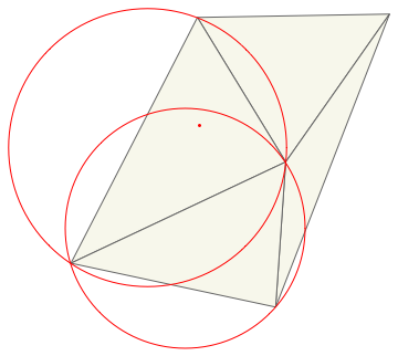
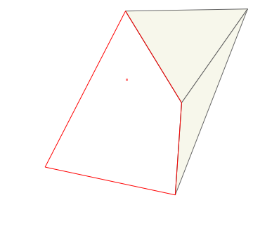
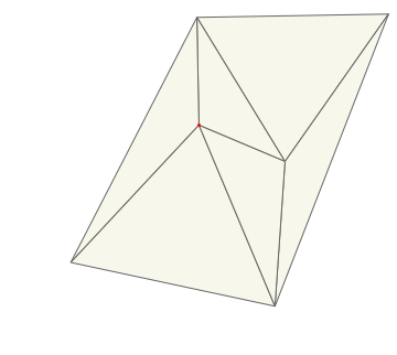
This point set can be converted to a mesh by any Delaunay triangulation method, the Bowyer-Watson algorithm is probably the simplest. It works by inserting one point at a time, removing any triangles whose circumcircle is encroached by the new point and re-tessellating the surrounding edges. A nice feature is that the algorithm has a direct analogue for tetrahedral meshes, triangles become tetrahedra, edges become faces and circumcircles become circumspheres.
Here's an illustration of how Bowyer/Watson proceeds to insert the point in red into the mesh:

And here is the Delaunay triangulation of the Armadillo point set:
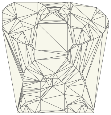
As you can see, Delaunay triangulation algorithms generate the convex hull of the input points. But we want a mesh that conforms to the shape boundary - one way to fix this is to sample the image at each triangle's centroid, if the sample lies outside the shape then simply throw away the triangle. This produces:
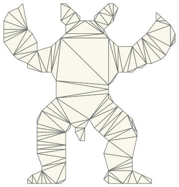
Much better! Now we have a reasonably good approximation of the input shape. Unfortunately, FEM simulations don't work well with long thin "sliver" triangles. This is due to interpolation error and because a small movement in one of the triangle's vertices leads to large forces, which leads to inaccuracy and small time steps [2].
Before we look at ways to improve triangle quality it's worth talking about how to measure it. One measure that works well in 2D is the ratio of the triangle's circumradius to it's shortest edge. A smaller ratio indicates a higher quality triangle, which intuitively seems reasonable, long skinny triangles have a large circumradius but one very short edge:
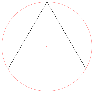
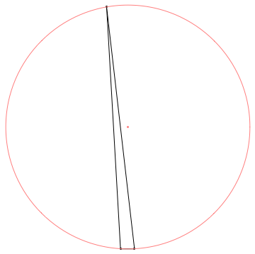
The triangle on the left, which is equilateral, has a ratio ~0.5 and is the best possible triangle by this measure. The triangle on the right has a ratio of ~8.7, note the circumcenter of sliver triangles tend to fall outside of the triangle itself.
Delaunay refinement
Methods such as Chew's algorithm and Ruppert's algorithm are probably the most well known refinement algorithms. They attempt to improve mesh quality while maintaining the Delaunay property (no vertex encroaching a triangle's circumcircle). This is typically done by inserting the circumcenter of low-quality triangles and subdividing edges.
Jonathon Shewchuk's "ultimate guide" has everything you need to know and there is Triangle, an open source tool to generate high quality triangulations.
Unfortunately these algorithms require an accurate polygonal boundary as input as the output is sensitive to the input segment lengths. They are also famously difficult to implement robustly and efficiently, I spent most of my time implementing Ruppert's algorithm only to find the next methods produced better results with much simpler code.
Variational Methods
Variational (energy based) algorithms improve the mesh through a series of optimization steps that attempt to minimize a global energy function. I adapted the approach in Variational Tetrahedral Meshing [3] to 2D and found it produced great results, this is the method I settled on so I'll go into some detail.
The algorithm proceeds as follows:
- Generate a set of uniformly distributed points interior to the shape P
- Generate a set of points on the boundary of the shape B
- Generate a Delaunay triangulation of P
- Optimize boundary points by moving them them to the average of their neighbours in B
- Optimize interior points by moving them to the centroid of their Voronoi cell (area weighted average of connected triangle circumcenters)
- Unless stopping criteria met, go to 3.
- Remove boundary sliver triangles
The core idea is that of repeated triangulation (3) and relaxation (4,5), it's a somewhat similar process to Lloyd's clustering, conincidentally the same algorithm I had used to generate surfel hierarchies for global illumination sims in the past.
Here's an animation of 7 iterations on the Armadillo, note the number of points stays the same throughout (another nice property):

It's interesting to see how much the quality improves after the very first step. Although Alliez et al. [3] don't provide any guarantees on the resulting mesh quality I found the algorithm works very well on a variety of input images with a fixed number of iterations.
This is the algorithm I ended up using but I'll quickly cover a couple of alternatives for completeness.
Structured Methods
These algorithms typically start by tiling interior space using a BCC (body centered cubic) lattice which is simply two interleaved grids. They then generate a Delaunay triangulation and throw away elements lying completely outside the region of interest.
As usual, handling boundaries is where the real challenge lies, Molino et al. [4] use a force based simulation to push grid points towards the boundary. Isosurface Stuffing [5] refines the boundary by directly moving vertices to the zero-contour of a signed distance field or inserts new vertices if moving the existing lattice nodes would generate a poor quality triangle.
Lattice based methods are typically very fast and don't suffer from the numerical robustness issues of algorithms that rely on triangulation. However if you plan on fracturing the mesh along element boundaries then this regular nature is exposed and looks quite unconvincing.
Simplification Methods
Another approach is to start with a very fine-grained mesh and progressively simplify it in the style of Progressive Meshes [6]. Barbara Cutler's thesis and associated paper discusses the details and very helpfully provides the resulting tetrahedral meshes, but the implementation appears to be considerably more complex than variational methods and relies on quite a few heuristics to get good results.
Simulation
Now the mesh is ready it's time for the fun part (apologies if you really love meshing). This simple simulation is using co-rotational linear FEM with a semi-implicit time-stepping scheme:
(Armadillo and Bunny images courtesy of the Stanford Scanning Respository)
Pre-built binaries for OSX/Win32 here: http://mmacklin.com/fem.zip
Source code is available on Github: https://github.com/mmacklin/sandbox/tree/master/projects/fem.
Refs:
[1] Matthias Müller, Jos Stam, Doug James, and Nils Thürey. Real time physics: class notes. In ACM SIGGRAPH 2008 classes http://www.matthiasmueller.info/realtimephysics/index.html
[2] Jonathan Richard Shewchuk. 2002. What Is a Good Linear Finite Element? Interpolation, Conditioning, Anisotropy, and Quality Measures, unpublished preprint. http://www.cs.berkeley.edu/~jrs/papers/elemj.pdf
[3] Pierre Alliez, David Cohen-Steiner, Mariette Yvinec, and Mathieu Desbrun. 2005. Variational tetrahedral meshing. ftp://ftp‑sop.inria.fr/prisme/alliez/vtm.pdf
[4] Molino, Bridson, et al. - 2003. A Crystalline, Red Green Strategy for Meshing Highly Deformable Objects with Tetrahedra http://www.math.ucla.edu/~jteran/papers/MBTF03.pdf
[5] François Labelle and Jonathan Richard Shewchuk. 2007. Isosurface stuffing: fast tetrahedral meshes with good dihedral angles. In ACM SIGGRAPH 2007 papers http://www.cs.berkeley.edu/~jrs/papers/stuffing.pdf
[6] Hugues Hoppe. 1996. Progressive meshes. http://research.microsoft.com/en-us/um/people/hoppe/pm.pdf
Implicit Springs
This is a quick post to document some work I did while writing a mass spring simulation using an implicit integrator. Implicit, or backward Euler integration is well described in David Baraff's Physically Based Modelling SIGGRAPH course and this post assumes some familiarity with it.
Springs are a workhorse in physical simulation, once you have unconditionally stable springs you can use them to model just about anything, from rigid bodies to drool and snot. For example, Industrial Light & Magic used a tetrahedral mesh with edge and altitude springs to model the damage to ships in Avatar (see Avatar: Bending Rigid Bodies).
If you sit down and try and implement an implicit integrator one of the first things you need is the Jacobian of the particle forces with respect to the particle positions and velocities. The rest of this post shows how to derive these Jacobians for a basic Hookean spring in a form ready to be plugged into a linear system solver (I use a hand-rolled conjugate gradient solver, see Jonathon Shewchuk's painless introduction for details, it is all of about 20 lines of code to implement).
\[\renewcommand{\v}[1]{\mathbf{#1}} \newcommand{\uv}[1]{\mathbf{\widehat{#1}}} \newcommand\ddx[1]{\frac{\partial#1}{\partial \v{x} }} \newcommand\dd[2]{\frac{\partial#1}{\partial #2}}\]
Vector Calculus Basics
In order to calculate the force Jacobians we first need to know how to calculate the derivatives of some basic geometric quantities with respect to a vector.
In general the derivative of a scalar valued function with respect to a vector is defined as the following row vector of partial derivatives:
\[ \ddx{f} = \begin{bmatrix} \dd{f}{x_i} & \dd{f}{x_j} & \dd{f}{x_k} \end{bmatrix}\]
And for a vector valued function with respect to a vector:
\[\ddx{\v{f}} = \begin{bmatrix} \dd{f_i}{x_i} & \dd{f_i}{x_j} & \dd{f_i}{x_k} \\ \dd{f_j}{x_i} & \dd{f_j}{x_j} & \dd{f_j}{x_k} \\ \dd{f_k}{x_i} & \dd{f_k}{x_j} & \dd{f_k}{x_k} \end{bmatrix}\]
Applying the first definition to the dot product of two vectors we can calculate the derivative with respect to one of the vectors:
\[\ddx{\v{x}^T \cdot \v{y}} = \v{y}^T \]
Note that I'll explicitly keep track of whether vectors are row or column vectors as it will help keep things straight later on.
The derivative of a vector magnitude with respect to the vector, gives the normalized vector transposed:
\[\ddx{|\v{x}|} = \left(\frac{\v{x}}{|\v{x}|}\right)^T = \uv{x}^T \]
The derivative of a normalized vector \(\v{\widehat{x}} = \frac{\v{x}}{|\v{x}|} \) can be obtained using the quotient rule:
\[\ddx{\uv{x}} = \frac{\v{I}|\v{x}| - \v{x}\cdot\uv{x}^T}{|\v{x}|^2}\]
Where \(\v{I}\) is the \(n\) x \(n\) identity matrix and n is the dimension of \(x\). The product of a column vector and a row vector \(\uv{x}\cdot\uv{x}^T\) is the outer product which is a \(n\) x \(n\) matrix that can be constructed using standard matrix multiplication definition.
Dividing through by \(|\v{x}|\) we have:
\[\ddx{\uv{x}} = \frac{\v{I} - \uv{x}\cdot\uv{x}^T}{\v{|x|}}\]
Jacobian of Stretch Force
Now we are ready to compute the Jacobian of the spring forces. Recall the equation for the elastic force on a particle \(i\) due to an undamped Hookean spring:
\[\v{F_s} = -k_s(|\v{x}_{ij}| - r)\uv{x}_{ij}\]
Where \(\v{x}_{ij} = \v{x}_i - \v{x}_j\) is the vector between the two connected particle positions, \(r\) is the rest length and \(k_s\) is the stiffness coefficient.
The Jacobian of this force with respect to particle \(i\)'s position is obtained by using the product rule for the two \(\v{x}_i\) dependent terms in \(\v{F_s}\):
\[\dd{\v{F_s}}{\v{x}_i} = -ks\left[(|\v{x}_{ij}| - r)\dd{\uv{x}_{ij}}{\v{x}_i} + \uv{x}_{ij}\dd{(|\v{x}_{ij}| - r)}{\v{x}_i}\right]\]
Using the previously derived formulas for the derivative of a vector magnitude and normalized vector we have:
\[\dd{\v{F_s}}{\v{x}_i} = -ks\left[(|\v{x}_{ij}| - r)\left(\frac{\v{I} - \uv{x}_{ij}\cdot \uv{x}_{ij}^T}{|\v{x}_{ij}|}\right) + \uv{x}_{ij}\cdot\uv{x}_{ij}^T\right]\]
Dividing the first two terms through by \(|\v{x}_{ij}|\):
\[\dd{\v{F_s}}{\v{x}_i} = -ks\left[(1 - \frac{r}{|\v{x}_{ij}|})\left(\v{I} - \uv{x}_{ij}\cdot \uv{x}_{ij}^T\right) + \uv{x}_{ij}\cdot \uv{x}_{ij}^T\right]\]
Due to the symmetry in the definition of \(\v{x}_{ij}\) we have the following force derivative with respect to the opposite particle:
\[\dd{\v{F_s}}{\v{x}_j} = -\dd{\v{F_s}}{\v{x}_i}\]
Jacobian of Damping Force
The equation for the damping force on a particle \(i\) due to a spring is:
\[\v{F_d} = -k_d\cdot\uv{x}(\v{v}_{ij}\cdot \uv{x}_{ij})\]
Where \(\v{v}_{ij} = \v{v}_i-\v{v}_j\) is the relative velocities of the two particles. This is the preferred formulation because it damps only relative velocity along the spring axis.
Taking the derivative with respect to \(\v{v}_i\):
\[\dd{\v{F_d}}{\v{v}_i} = -k_d\cdot\uv{x}\cdot\uv{x}^T\]
As with stretching, the force on the opposite particle is simply negated:
\[\dd{\v{F_d}}{\v{v}_j} = -\dd{\v{F_d}}{\v{v}_i} \]
Note that implicit integration introduces it's own artificial damping so you might find it's not necessary to add as much additional damping as you would with an explicit integration scheme.
I'll be going into more detail about implicit methods and FEM in subsequent posts, stay tuned!
Refs
[Baraff Witkin] - Physically Based Modelling, SIGGRAPH course
[Baraff Witkin] - Large Steps in Cloth Simulation
[N. Joubert] - An Introduction to Simulation
[D Prichard] - Implementing Baraff and Witkin's Cloth Simulation
[Choi] - Stable but Responsive Cloth
Numerical Recipes, 3rd edition 2007 - ch17.5
New Look
Hi all, welcome to my new site. I've moved to my own hosting and have updated a few things - a new theme and a switch to MathJax for equation rendering. Apologies to RSS readers who will now see only a bunch of Latex code, but it is currently by far the easiest way to put decent looking equations in a web page.
It's been a little over a year since I started working at NVIDIA and not coincidentally, since my last blog post. I'm really enjoying working more on the simulation side of things, it makes a nice change from pure rendering and the PhysX team is full of über-talented people who I'm learning a lot from.
I've got some simulation related posts (from a graphics programmer's perspective) planned over the next few months, I hope you enjoy them!